Frequencies

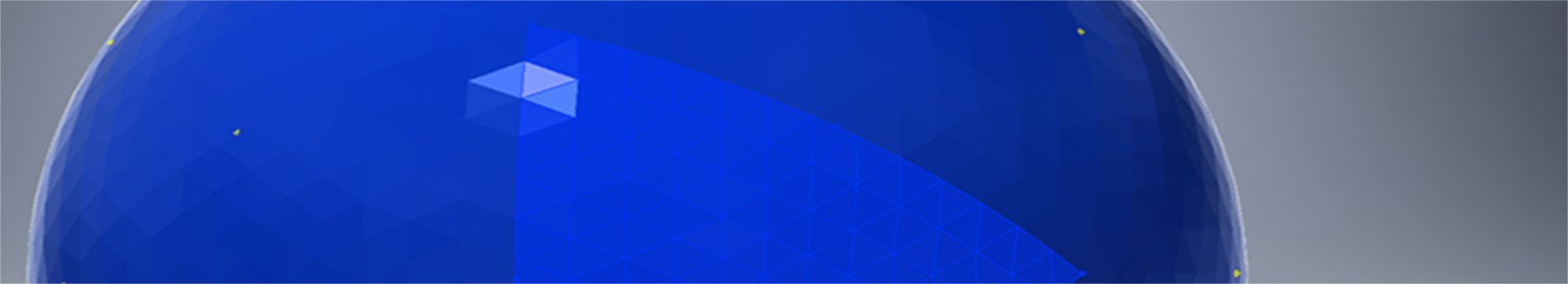
As previously discussed frequency is the subdivision of each parent tile in a geodesic tessellation. In this case we are working with an icosahedron base. Our parent tile is therefore the spheroidal patch defined by the 3 corners of an equilateral triangular face of an icosahedron inscribed in a sphere. For our purposes here we will be using a Patch Map. This map is simply a 2d, not to scale, map describing the relative location of varying edge lengths distributed across the patch.

With the higher levels of frequency easily available using Rose Geodesics it is helpful to take a deeper look at the repetitive 3 fold nature of tessellation in this instance. Doing so will be helpful in understanding the choices made for naming conventions as well as simplify mapping higher frequencies.

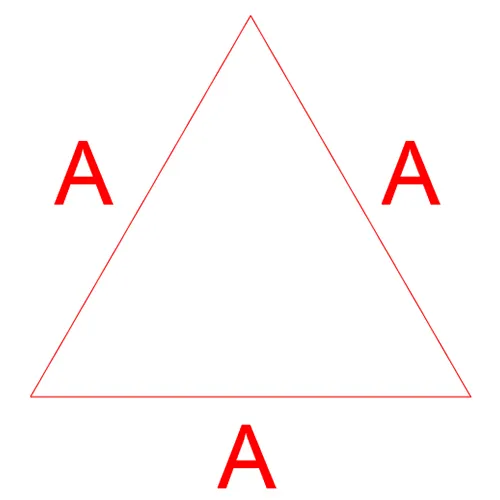
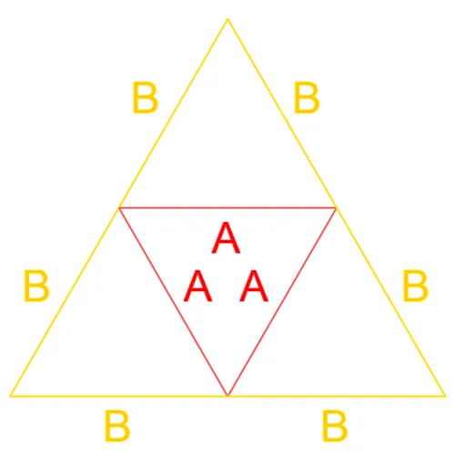
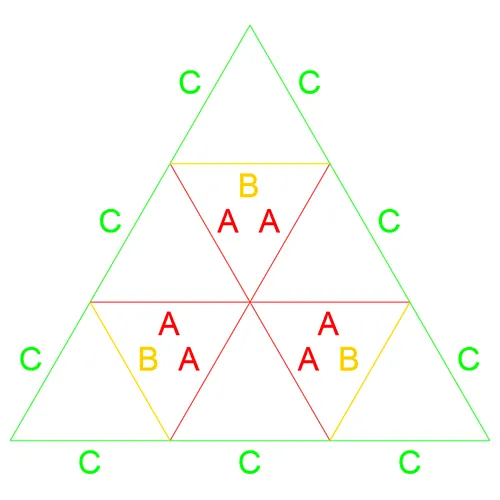
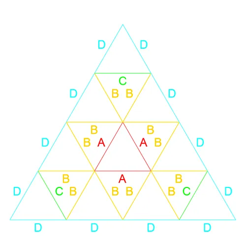
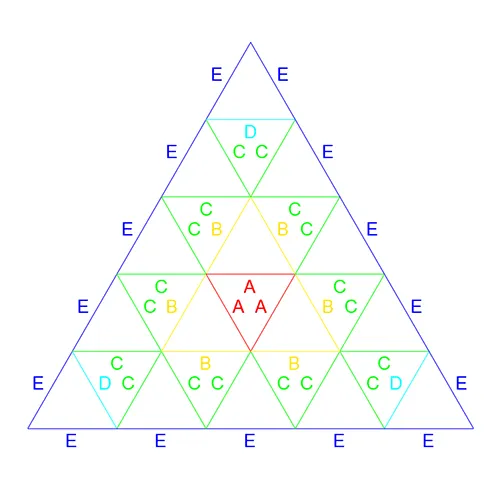
Looking at the Rose1V, Rose2V, and Rose3V Patch Maps we can observe the fundamental base of the 3 map categories, Category 1 (C1), Category 2 (C2), and Category 3 (C3). The easiest way to visually recognize which map belongs to what category is to observe the faces defined by the A edge lengths. the Rose1V Patch map belongs to C1 as the AAA length face points in the same general direction as the original icosahedron face being subdivided. In the case of the Rose1V this is trivial as there is no subdivision however this becomes significant with higher frequencies. C2 frequencies are those that have faces defined by the AAA edge lengths which point in the opposite direction as the original icosahedron face. This can be see with the Rose2V Patch Map. Finally the C3 maps are defined by multiple AA faces, AAB and AAC, as can be seen with the Rose3V Patch Map.

Fortunately the categories are cyclical and simply repeat. Therefore determining which category a map will belong to can be determined with a simple modulus function. if Rose(n)V modulus 3 =1 then Rose(n)V is C1, Rose(n)V modulus 3 = 2 is C2, Rose(n)V modulus 3 = 0 is C3. Let us use this to move into the higher level of frequencies. Rose4V modulus 3 = 1 indicating C1, Rose5V modulus 3 = 2 indicating C2, and Rose6V modulus 3 = 0 indicating C3. This can be seen with the Rose4V, Rose5V, and Rose 6V Patch Maps.

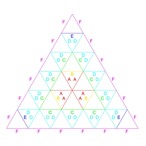
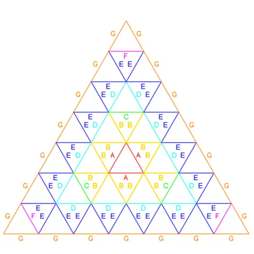
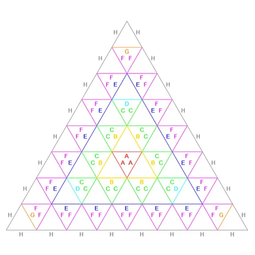
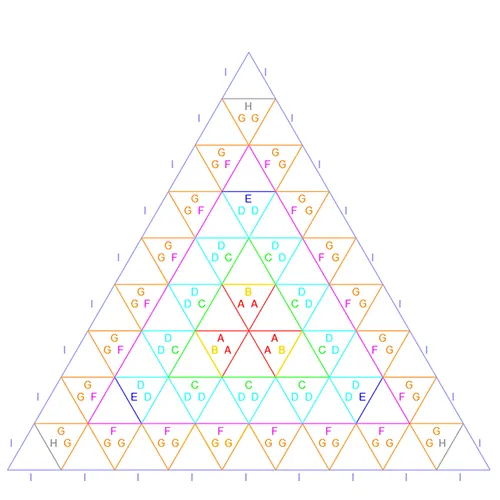
Arranging the patch maps in columns according to categories the evolution of maps becomes clear. C1, Rose1V 4V 7V, remains on the left column. C2 is on center, Rose2V 5V 8V. The right column, Rose3V 6V 9V, all belongs to C3. As expected the centers of each category remains consistent. Due to naming conventions utilized each frequency step in the categories simply adds a new layer of 3 new components. The base of each map remains the same. Alternatively, when viewed, a higher level map from a category shows each lower frequency map from within the same category embedded within itself. For example lets review Category 1. Looking at the Rose7V Patch Map we can see the Rose4V Patch Map by excluding E, F, and G components. Likewise removing the B, C, and D components from the Rose4V Patch maps leaves the Rose1V Patch Map. This is consistent across all 3 categories and a driving factor in the naming convention.

It is important to note that the scale factors of these edge components are not consistent across frequencies. The links to the left lead to details and images about various frequency Rose Geodesics. These details include patch maps, edge length factors (for scaling up size of the geodesic), and a variety of full and partial geodesic models.