The Buckminster Fuller Process
BF Geodesics can function with any Platonic solid. BF’s process is most commonly used with, the highest order Platonic sold, the Icosahedron. This explanation will, for easiest comparison, stick to the most commonly recognized approach. The Icosahedron is a logical starting point as it is the closest uniform shape to the sphere, in which it is inscribed, as possible having all faces being identical equilateral triangles. Ultimately the goal is to subdivide an equilateral triangular face into multiple smaller triangular faces across the spherical surface. Each of these sub-triangular faces are also inscribed inside the same sphere. Maintaining the best possible uniformity and equilateral triangle approximation of these sub-triangles improves the result. This subdivision is then used for tessellation across the sphere which then better approximates the sphere using straight line segments.
Frequency is the term for the degree in which the faces, or patches, are subdivided before being tessellated across the spherical surface. Each degree of frequency equates to the number of triangle edges that the original icosahedron edges are broken into. An Icosahedron in terms of geodesics is rereferred to as a 1V tessellation. The 2nd degree of tessellation would the be called a 2V having 2 edge lengths, the 3rd a 3V, and so on. The method for subdivision is the point where Rose Geodesics diverge from the BF process. The terminology shall remain the same for both the BF and Rose geodesics however we shall precede the frequency with BF or Rose to identify each process more easily. For the sake of easy comparison lets review BF’s process, as simply as possible and, not specifically by the actual BF route.
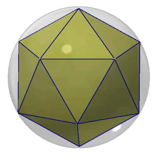
The simplest explanation of a BF geodesic would be the BF1V. This would yield an icosahedron inscribed inside a sphere (Fig 1.) As a wireframe approximation of a sphere every component would be of equal length and the model is rough. Obviously this isn’t quite enough to explain the full process so lets move to BF2V.
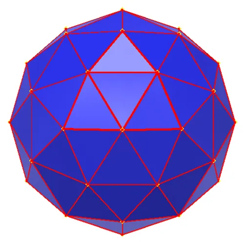
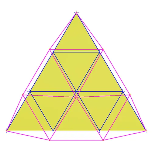
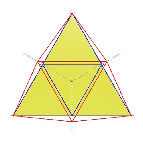
To keep the picture as clear as possible lets look at a single face of the Icosahedron. This is shown in figure 2 as the yellow equilateral triangle. Now BF cleverly decided to equally divide the edges into 2 parts for a BF2V geodesic. At that point edge nodes are used to draw a triangular grid (blue Lines in Fig. 2) on the face. This grid is the layout for a 2D representation of the patch layout. The edge nodes were then used to draw an axis from the center of the sphere (Fig. 2 as faint blue lines and dotted behind the face) through the node. A new node was then established on the edge of the sphere patch where the axis intersected the sphere. Each node on the spherical surface was then used to layout a network of new triangular faces as shown in red on Fig. 2. It is important to observe that this network is not planar. Lines between nodes are straight lines but the nodes do lay on the curvature of the bounding sphere. Additionally note that there are now 2 segment lengths between the nodes and that only the central triangular face is now equilateral. The BF2V tessellation across the sphere yields a better approximation of the sphere. This can be seen with a BF2V in Fig. 3. Note the edges, red lines, from a single patch are shown thicker in Fig 3 for clarity. While the BF2V starts to demonstrate the BF process we should look a little deeper.
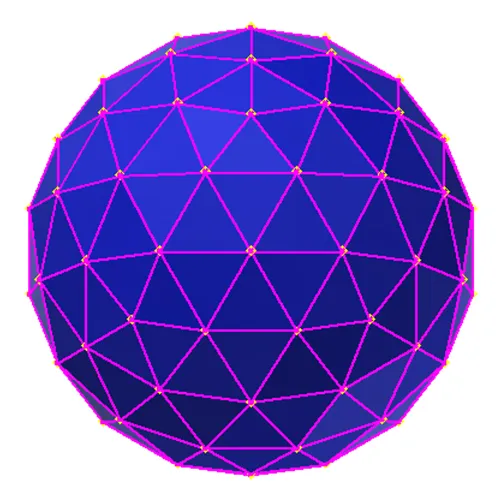
The BF3V is the first tessellation which has nodes, 1 in this case, inside the patch boundaries (Fig. 4.) All nodes in the BF geodesics are created in the same fashion being projected from the planar surface to the spherical surface. Interestingly this is also the last of the BF frequencies which has the same number, 3, of distinct edge lengths between nodes as the frequency. As can be seen in in Figure 5 the approximation of the sphere vastly improves with each increase in frequency. Unfortunately as we move to BF4V and beyond the increase in unique edge lengths grows nonlinearly.